You have data resulting from an aerobic fitness study, and you want to predict the oxygen uptake from several continuous variables.
1. Select Help > Sample Data Folder and open Fitness.jmp .
2. Select Analyze > Fit Model . Note that the Personality box is empty.
3. Select Oxy and click Y .
When you specify a continuous response, the Personality defaults to Standard Least Squares, but you are free to choose another personality. Also, the Emphasis defaults to Effect Leverage.
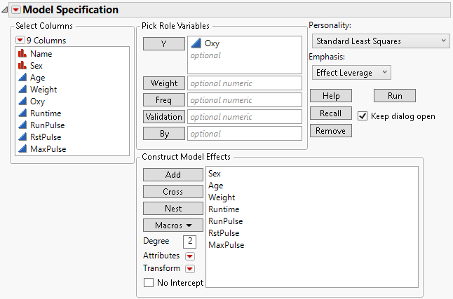
4. Press Ctrl and select Sex , Age , Weight , Runtime , RunPulse , RstPulse , and MaxPulse . Click Add to add these to the Construct Model Effects list. Note that you can select Keep dialog open if you want to have this window available later on. Your Model Specification window should appear as shown in Figure 2.1.
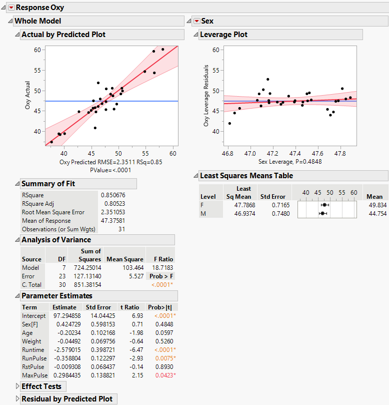
5. Click Run . Figure 2.2 gives a partial view of the report.
Figure 2.1 Model Specification Window for Fitness Regression Model

Figure 2.2 Partial View of Standard Least Squares Report for Fitness Data

The plot and reports for the whole model appear in the left-most report column. The columns to the right show leverage plots for each of the effects that you specified in the model. Due to space limitations, Figure 2.2 shows only the column for Sex , but the report shows columns for the other six effects as well. The red triangle menus contain additional options that add reports and plots to the report window. For more information about the Standard Least Squares report window, see “Fit Least Squares Report” .
Looking at the p -values in the Parameter Estimates report, you can see that Runtime , RunPulse , and MaxPulse appear to be significant predictors of oxygen uptake. The next step might be to reduce the model by removing insignificant predictors. See “Stepwise Regression Models” .